
Cloud Cost Optimization Framework
Table of contents
- Graph-Based Cloud Cost Optimization
- Introduction
- The Problem: Post-Deployment Optimization
- Our Approach: Design-Time Cost Intelligence
- System Architecture
- Core Components
- Technical Implementation
- End-to-End Flow
- Conclusion
Graph-Based Cloud Cost Optimization
Introduction
Cloud computing has revolutionized how we deploy and manage applications, but with this flexibility comes the challenge of managing costs effectively. In this post, I’ll explore an innovative approach to cloud cost optimization using graph theory, mathematical modeling, and agentic AI. We’ll look at how representing cloud resources as a graph can help make smarter decisions about resource allocation and cost management — before deployment, not after.
The Problem: Post-Deployment Optimization
Most cloud cost optimization happens after deployment, when architecture choices are already fixed. Organizations typically discover cost overruns through monthly billing surprises, leaving them with limited options: accept the costs, undertake expensive re-architecture efforts, or compromise on performance and reliability.
In ETL/ELT pipelines and multi-cloud data platforms, the real cost drivers are decided much earlier during the design phase:
- Compute and Engine Selection: The choice between different compute instance types, serverless functions, or managed services fundamentally determines the cost baseline
- Regions and Data Movement: Data transfer costs between regions and across cloud providers can exceed compute costs in data-intensive workloads
- Network and Storage Dependencies: The topology of how services connect and where data resides creates cascading cost implications
- Performance and Reliability Constraints: SLA requirements, latency bounds, and availability targets constrain the solution space and influence costs
Our Approach: Design-Time Cost Intelligence
Our approach shifts cost optimization to design time. By combining graph-based resource modeling with agentic AI for continuous cost intelligence gathering, we enable teams to explore and optimize their cloud architecture before committing infrastructure resources.
System Architecture
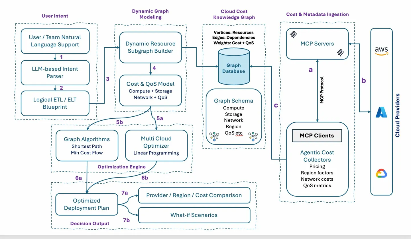
The system comprises four integrated layers working together to deliver design-time cost optimization:
| Layer | Purpose | Key Components |
|---|---|---|
| User Intent | Natural language interface for expressing pipeline requirements | NL Support, Intent Parser, Blueprint Generator |
| Cloud Cost Knowledge Graph | Unified cost-aware representation of multi-cloud resources | Graph Database, Schema Definitions |
| Cost & Metadata Ingestion | Continuous collection and normalization of cloud pricing data | MCP Servers, MCP Clients, Agentic Collectors |
| Dynamic Graph Modeling | Real-time subgraph construction and optimization | Subgraph Builder, Cost Model, Optimization Engine |
Core Components
1. User Intent Processing
The User Intent layer transforms natural language descriptions of ETL pipelines into structured, optimizable blueprints.
Natural Language Interface
Teams describe their pipeline requirements in natural language, including:
- Data sources and destinations
- Transformation logic and processing requirements
- Provider or region preferences and constraints
- Performance and reliability requirements
- Budget constraints or optimization targets
Example Input:
“We need a daily ETL pipeline that extracts sales data from our PostgreSQL database in US-East, transforms it using Spark for aggregations and joins, and loads the results into BigQuery for our analytics team. The pipeline should complete within 4 hours and we prefer to minimize cross-cloud data transfer costs.”
LLM-Based Intent Parser
The intent parser (Step 1 in the flow) uses large language models to:
- Extract structured requirements from natural language descriptions
- Identify explicit and implicit constraints
- Recognize domain-specific terminology and map to technical specifications
- Handle ambiguity through clarifying questions or reasonable defaults
- Validate completeness of the specification
Parser Outputs:
- Source systems and connection requirements
- Target systems and data models
- Transformation operations and their dependencies
- QoS constraints (latency, throughput, availability)
- Cost optimization preferences
Logical ETL/ELT Blueprint
The blueprint generator (Step 2) produces a logical representation of the pipeline that is:
- Provider-agnostic: Describes what needs to happen, not how
- Constraint-complete: Captures all requirements and preferences
- Graph-compatible: Structured for mapping to the knowledge graph
The blueprint specifies:
- Logical data flow stages
- Transformation semantics
- Dependency relationships
- Quality and performance gates
2. Cloud Cost Knowledge Graph
The Cloud Cost Knowledge Graph serves as the unified representation of cloud resources across providers, capturing costs, dependencies, and quality of service attributes.
Graph Structure
The graph models cloud infrastructure with three core elements:
| Element | Representation | Examples |
|---|---|---|
| Vertices (V) | Cloud resources | VMs, storage buckets, networks, managed services |
| Edges (E) | Dependencies and connections | Data flows, network links, service bindings |
| Weights | Cost + QoS attributes | Hourly costs, latency, bandwidth, availability |
This structure enables the system to reason about resource relationships and optimize across the entire infrastructure topology, not just individual resources.
Graph Schema
The graph schema defines vertex and edge types for comprehensive cloud resource modeling:
Compute Vertices:
- Instance types (families, sizes, generations)
- Serverless functions (memory configurations, execution limits)
- Container services (orchestration platforms, node pools)
- Managed compute services (EMR, Dataproc, Synapse)
Storage Vertices:
- Object storage (tiers, lifecycle policies)
- Block storage (IOPS, throughput classes)
- Database services (instance classes, storage engines)
- Data warehouse services (compute/storage separation)
Network Vertices:
- Virtual networks (VPCs, subnets)
- Load balancers (layer 4/7, regional/global)
- CDN endpoints and edge locations
- VPN and interconnect services
Region Vertices:
- Geographic locations
- Availability zones
- Edge locations
QoS Attributes:
- Latency metrics (intra-region, inter-region, cross-cloud)
- Availability SLAs
- Durability guarantees
- Throughput limits
3. Cost & Metadata Ingestion
The Cost & Metadata Ingestion layer implements an agentic architecture for continuous collection, normalization, and updating of pricing data from cloud providers.
MCP Architecture
The Model Context Protocol (MCP) provides a standardized interface for AI agents to interact with cloud provider APIs:
MCP Servers:
- Expose cloud provider APIs through a unified protocol
- Handle authentication and rate limiting
- Provide consistent data models across providers
- Support both real-time queries and batch updates
MCP Clients:
- Connect to multiple MCP servers simultaneously
- Orchestrate data collection workflows
- Handle failures and retries gracefully
- Maintain session state for complex queries
MCP Protocol:
- Bidirectional communication between servers and clients
- Structured message formats for requests and responses
- Support for streaming updates and subscriptions
- Context passing for multi-step operations
Agentic Cost Collectors
The agentic cost collectors autonomously gather and normalize pricing information:
| Collector Type | Data Collected | Update Frequency |
|---|---|---|
| Pricing | On-demand, reserved, spot prices; commitment discounts | Hourly for spot, daily for others |
| Region Factors | Regional price multipliers, availability premiums | Weekly |
| Network Costs | Data transfer rates (intra-region, inter-region, internet egress) | Daily |
| QoS Metrics | Historical latency, availability, throughput measurements | Continuous |
Multi-Cloud Support:
- AWS (a): EC2, S3, RDS, Lambda, EMR pricing via AWS Pricing API
- Azure (b): VMs, Blob Storage, SQL Database, Functions via Azure Retail Prices API
- GCP (c): Compute Engine, Cloud Storage, BigQuery via Cloud Billing Catalog API
The agents maintain a normalized cost model that enables direct comparison across providers despite different pricing structures (per-second vs. per-hour, tiered vs. flat-rate, etc.).
4. Dynamic Graph Modeling
The Dynamic Graph Modeling layer constructs and enriches subgraphs specific to each optimization request.
Dynamic Resource Subgraph Builder
The subgraph builder (Step 3) maps the logical blueprint to actual cloud resources:
Mapping Process:
- Parse the logical blueprint stages
- Identify candidate resources for each stage from the knowledge graph
- Filter candidates based on explicit constraints (regions, providers, resource types)
- Construct edges representing valid data flows between candidates
- Attach cost and QoS weights from the knowledge graph
Example Subgraph Construction:
For a Spark transformation stage requiring:
- Minimum 32 GB memory per executor
- US region
- Support for S3 and GCS connectivity
The builder identifies candidates across:
- AWS EMR clusters with various instance types
- GCP Dataproc clusters with various machine types
- Azure HDInsight clusters with various VM sizes
Each candidate becomes a vertex in the subgraph with edges to compatible upstream and downstream resources.
Cost & QoS Model
The Cost & QoS Model (Step 4) enriches the subgraph with comprehensive cost calculations:
Compute + Storage Costs:
- Instance/service hourly rates
- Storage capacity and operation costs
- Data processing costs (per-byte or per-query)
- Managed service premiums
Network + QoS Costs:
- Data ingress (typically free)
- Data egress (tiered pricing)
- Cross-region transfer costs
- Cross-cloud transfer costs
- Private connectivity premiums
The model combines these into edge weights that represent the true cost of each path through the infrastructure graph.
5. Optimization Engine
The Optimization Engine applies mathematical optimization techniques to find the best resource allocation.
Graph Algorithms
Shortest Path (Step 5b): The system applies Dijkstra’s algorithm to find the minimum cost path through the resource graph:
- Path represents the end-to-end pipeline configuration
- Edge weights combine resource costs and QoS penalties
- Constraints are encoded as edge exclusions or weight modifications
Min Cost Flow: For complex pipelines with multiple parallel paths or resource sharing:
- Models the problem as a minimum cost flow network
- Supports capacity constraints on resources
- Handles multi-commodity flows for different data streams
- Finds globally optimal resource allocation
Multi-Cloud Optimizer
Linear Programming (Step 5a): For multi-cloud optimization with complex constraints, the system formulates and solves linear programs:
Decision Variables:
- Resource allocation amounts (xᵢⱼ): amount of resource i allocated to provider j
Objective Function:
- Minimize total cost: Σᵢ Σⱼ Cᵢⱼ × xᵢⱼ
Constraints:
- Demand satisfaction: Σⱼ xᵢⱼ ≥ Dᵢ for all resource types i
- Capacity limits: Σᵢ xᵢⱼ ≤ Kⱼ for all providers j
- Non-negativity: xᵢⱼ ≥ 0 for all i, j
- QoS constraints: latency, availability thresholds
- Policy constraints: data residency, vendor preferences
6. Decision Output
The Decision Output layer presents optimization results in actionable formats.
Optimized Deployment Plan (Step 6a): The primary output is a concrete deployment specification including:
- Specific resources to provision (instance types, sizes, counts)
- Configuration parameters for each resource
- Network topology and connectivity requirements
- Estimated costs broken down by component and provider
Provider/Region/Cost Comparison (Steps 6b, 7a): Comparative analysis showing:
- Cost breakdown by cloud provider
- Regional cost variations
- Trade-offs between cost, performance, and reliability
- Sensitivity analysis for key parameters
What-If Scenarios (Step 7b): Interactive exploration of alternatives:
- Impact of changing constraints (e.g., relaxing latency requirements)
- Cost implications of provider lock-in vs. multi-cloud
- Reserved capacity vs. on-demand trade-offs
- Scaling scenarios and cost projections
Technical Implementation
1. Graph-Based Resource Modeling
2. Cost Modeling Framework
3. Optimization Techniques
A. Shortest Path Algorithm
B. Multi-Cloud Optimization
End-to-End Flow
The complete optimization flow progresses through seven steps:
| Step | Component | Action |
|---|---|---|
| 1 | LLM Intent Parser | Parse natural language requirements |
| 2 | Blueprint Generator | Create logical ETL/ELT blueprint |
| 3 | Subgraph Builder | Construct resource subgraph from knowledge graph |
| 4 | Cost & QoS Model | Enrich subgraph with cost and quality weights |
| 5a | Multi-Cloud Optimizer | Apply linear programming for multi-provider optimization |
| 5b | Graph Algorithms | Apply shortest path / min cost flow algorithms |
| 6a | Deployment Plan | Generate optimized deployment specification |
| 6b/7a | Comparison | Produce provider/region/cost comparisons |
| 7b | What-If Analysis | Enable scenario exploration |
Throughout this flow, the Cost & Metadata Ingestion layer continuously updates the knowledge graph with current pricing, ensuring optimization decisions reflect real-world costs.
Conclusion
Graph-based cloud cost optimization, enhanced with agentic AI for continuous cost intelligence, provides a powerful framework for managing cloud costs effectively. By shifting optimization to design time, teams can:
- Explore cost implications before committing resources
- Compare multi-cloud options systematically
- Understand trade-offs between cost, performance, and reliability
- Make informed decisions based on current, normalized pricing data
By combining graph theory with advanced optimization techniques and natural language interfaces, we enable teams to make better decisions about resource allocation and cost management — transforming cloud cost optimization from a reactive, post-deployment activity into a proactive, design-time capability.